Selecting Collections
This tutorial shows how to select a collection and visualize a cube:
[1]:
import cubo
import xarray as xr
This code creates a cube with an edge size of 64 pixels from Sentinel-2 and apply a cloud coverage filter of 40 percent. Get just the RGB bands:
[2]:
da = cubo.create(
    lat=47.848151988493385,
    lon=13.379491178028564,
    collection="sentinel-2-l2a",
    bands=["B02","B03","B04"],
    start_date="2020-01-01",
    end_date="2021-01-01",
    edge_size=64,
    resolution=10,
    query={"eo:cloud_cover": {"lt": 40}}
)
da
[2]:
<xarray.DataArray 'sentinel-2-l2a' (time: 46, band: 3, y: 64, x: 64)>
dask.array<fetch_raster_window, shape=(46, 3, 64, 64), dtype=float64, chunksize=(1, 1, 64, 64), chunktype=numpy.ndarray>
Coordinates: (12/46)
  * time                                     (time) datetime64[ns] 2020-01-01...
    id                                       (time) <U54 'S2B_MSIL2A_20200101...
  * band                                     (band) <U3 'B02' 'B03' 'B04'
  * x                                        (x) float64 3.784e+05 ... 3.791e+05
  * y                                        (y) float64 5.301e+06 ... 5.3e+06
    s2:medium_proba_clouds_percentage        (time) float64 0.3489 ... 4.911
    ...                                       ...
    title                                    (band) <U20 'Band 2 - Blue - 10m...
    proj:transform                           object {0.0, 300000.0, 5400000.0...
    common_name                              (band) <U5 'blue' 'green' 'red'
    center_wavelength                        (band) float64 0.49 0.56 0.665
    full_width_half_max                      (band) float64 0.098 0.045 0.038
    epsg                                     <U10 'EPSG:32633'
Attributes:
    collection:           sentinel-2-l2a
    stac:                 https://planetarycomputer.microsoft.com/api/stac/v1
    epsg:                 EPSG:32633
    resolution:           10
    edge_size:            64
    central_lat:          47.848151988493385
    central_lon:          13.379491178028564
    central_y:            5300694.38448788
    central_x:            378764.6058600877
    time_coverage_start:  2020-01-01
    time_coverage_end:    2021-01-01
xarray.DataArray
'sentinel-2-l2a'
- time: 46
- band: 3
- y: 64
- x: 64
- dask.array<chunksize=(1, 1, 64, 64), meta=np.ndarray>
Array Chunk Bytes 4.31 MiB 32.00 kiB Shape (46, 3, 64, 64) (1, 1, 64, 64) Count 414 Tasks 138 Chunks Type float64 numpy.ndarray - time(time)datetime64[ns]2020-01-01T10:03:19.024000 ... 2...
array(['2020-01-01T10:03:19.024000000', '2020-01-06T10:04:01.024000000', '2020-01-16T10:03:41.024000000', '2020-02-08T10:11:51.024000000', '2020-03-16T10:00:21.024000000', '2020-03-19T10:10:21.024000000', '2020-03-24T10:06:49.024000000', '2020-04-03T10:05:49.024000000', '2020-04-05T10:00:21.024000000', '2020-04-08T10:10:21.024000000', '2020-04-10T10:00:29.024000000', '2020-04-23T10:05:49.024000000', '2020-04-25T10:00:31.024000000', '2020-04-30T10:00:19.024000000', '2020-05-08T10:10:31.024000000', '2020-05-15T10:00:31.024000000', '2020-05-18T10:10:31.024000000', '2020-06-02T10:05:59.024000000', '2020-06-12T10:05:59.025000000', '2020-06-24T10:00:31.024000000', '2020-06-27T10:10:31.024000000', '2020-07-07T10:10:31.024000000', '2020-07-09T10:00:29.024000000', '2020-07-12T10:05:59.024000000', '2020-07-22T10:05:59.024000000', '2020-07-27T10:10:31.024000000', '2020-07-29T10:00:29.024000000', '2020-08-01T10:05:59.024000000', '2020-08-06T10:10:31.024000000', '2020-08-08T10:00:29.024000000', '2020-08-11T10:05:59.024000000', '2020-08-13T10:00:31.024000000', '2020-08-16T10:10:31.024000000', '2020-08-21T10:05:59.024000000', '2020-08-26T10:10:31.024000000', '2020-09-05T10:10:31.024000000', '2020-09-12T10:00:31.024000000', '2020-09-15T10:10:31.025000000', '2020-09-20T10:06:49.024000000', '2020-09-22T10:00:31.024000000', '2020-09-27T10:00:29.024000000', '2020-11-06T10:02:19.024000000', '2020-11-14T10:13:01.024000000', '2020-11-29T10:13:59.024000000', '2020-12-29T10:13:29.024000000', '2020-12-31T10:04:11.024000000'], dtype='datetime64[ns]') - id(time)<U54'S2B_MSIL2A_20200101T100319_R122...
array(['S2B_MSIL2A_20200101T100319_R122_T33UUP_20201002T214037', 'S2A_MSIL2A_20200106T100401_R122_T33UUP_20201002T233508', 'S2A_MSIL2A_20200116T100341_R122_T33UUP_20201002T191948', 'S2A_MSIL2A_20200208T101151_R022_T33UUP_20201001T084006', 'S2A_MSIL2A_20200316T100021_R122_T33UUP_20201010T094601', 'S2A_MSIL2A_20200319T101021_R022_T33UUP_20201012T164319', 'S2B_MSIL2A_20200324T100649_R022_T33UUP_20201018T203745', 'S2B_MSIL2A_20200403T100549_R022_T33UUP_20200924T212414', 'S2A_MSIL2A_20200405T100021_R122_T33UUP_20200925T021631', 'S2A_MSIL2A_20200408T101021_R022_T33UUP_20200925T120557', 'S2B_MSIL2A_20200410T100029_R122_T33UUP_20200925T201646', 'S2B_MSIL2A_20200423T100549_R022_T33UUP_20200921T200025', 'S2A_MSIL2A_20200425T100031_R122_T33UUP_20200922T004857', 'S2B_MSIL2A_20200430T100019_R122_T33UUP_20200922T183401', 'S2A_MSIL2A_20200508T101031_R022_T33UUP_20200921T001025', 'S2A_MSIL2A_20200515T100031_R122_T33UUP_20200918T065533', 'S2A_MSIL2A_20200518T101031_R022_T33UUP_20200910T022254', 'S2B_MSIL2A_20200602T100559_R022_T33UUP_20200825T220006', 'S2B_MSIL2A_20200612T100559_R022_T33UUP_20200909T150432', 'S2A_MSIL2A_20200624T100031_R122_T33UUP_20200823T221236', ... 'S2B_MSIL2A_20200801T100559_R022_T33UUP_20200815T190855', 'S2A_MSIL2A_20200806T101031_R022_T33UUP_20200815T051443', 'S2B_MSIL2A_20200808T100029_R122_T33UUP_20200815T123356', 'S2B_MSIL2A_20200811T100559_R022_T33UUP_20200814T182203', 'S2A_MSIL2A_20200813T100031_R122_T33UUP_20200815T000738', 'S2A_MSIL2A_20200816T101031_R022_T33UUP_20200919T022032', 'S2B_MSIL2A_20200821T100559_R022_T33UUP_20200919T022031', 'S2A_MSIL2A_20200826T101031_R022_T33UUP_20200909T150432', 'S2A_MSIL2A_20200905T101031_R022_T33UUP_20200908T034143', 'S2A_MSIL2A_20200912T100031_R122_T33UUP_20200918T133658', 'S2A_MSIL2A_20200915T101031_R022_T33UUP_20200918T101612', 'S2B_MSIL2A_20200920T100649_R022_T33UUP_20200922T235721', 'S2A_MSIL2A_20200922T100031_R122_T33UUP_20201028T031042', 'S2B_MSIL2A_20200927T100029_R122_T33UUP_20200929T024741', 'S2B_MSIL2A_20201106T100219_R122_T33UUP_20201107T150945', 'S2A_MSIL2A_20201114T101301_R022_T33UUP_20201116T031518', 'S2B_MSIL2A_20201129T101359_R022_T33UUP_20201130T021404', 'S2B_MSIL2A_20201229T101329_R022_T33UUP_20201229T175849', 'S2A_MSIL2A_20201231T100411_R122_T33UUP_20210101T041851'], dtype='<U54') - band(band)<U3'B02' 'B03' 'B04'
array(['B02', 'B03', 'B04'], dtype='<U3')
- x(x)float643.784e+05 3.784e+05 ... 3.791e+05
array([378440., 378450., 378460., 378470., 378480., 378490., 378500., 378510., 378520., 378530., 378540., 378550., 378560., 378570., 378580., 378590., 378600., 378610., 378620., 378630., 378640., 378650., 378660., 378670., 378680., 378690., 378700., 378710., 378720., 378730., 378740., 378750., 378760., 378770., 378780., 378790., 378800., 378810., 378820., 378830., 378840., 378850., 378860., 378870., 378880., 378890., 378900., 378910., 378920., 378930., 378940., 378950., 378960., 378970., 378980., 378990., 379000., 379010., 379020., 379030., 379040., 379050., 379060., 379070.]) - y(y)float645.301e+06 5.301e+06 ... 5.3e+06
array([5301010., 5301000., 5300990., 5300980., 5300970., 5300960., 5300950., 5300940., 5300930., 5300920., 5300910., 5300900., 5300890., 5300880., 5300870., 5300860., 5300850., 5300840., 5300830., 5300820., 5300810., 5300800., 5300790., 5300780., 5300770., 5300760., 5300750., 5300740., 5300730., 5300720., 5300710., 5300700., 5300690., 5300680., 5300670., 5300660., 5300650., 5300640., 5300630., 5300620., 5300610., 5300600., 5300590., 5300580., 5300570., 5300560., 5300550., 5300540., 5300530., 5300520., 5300510., 5300500., 5300490., 5300480., 5300470., 5300460., 5300450., 5300440., 5300430., 5300420., 5300410., 5300400., 5300390., 5300380.]) - s2:medium_proba_clouds_percentage(time)float640.3489 5.747 13.82 ... 9.511 4.911
array([ 0.348905, 5.747249, 13.820124, 5.14272 , 0.089794, 0.074748, 0.618072, 1.500922, 0.073965, 0.043816, 1.270113, 0.056728, 2.716188, 1.177769, 0.142521, 15.790294, 0.18199 , 1.40714 , 0.098162, 2.706701, 0.535921, 4.012835, 9.326182, 4.50226 , 6.191069, 0.599982, 8.968821, 0.133178, 1.198564, 0.289764, 0.457776, 4.717574, 1.160753, 0.053547, 1.262791, 2.194467, 1.610077, 0.078832, 1.158529, 0.323638, 1.323876, 3.006202, 2.746796, 1.432766, 9.510832, 4.911026]) - s2:cloud_shadow_percentage(time)float646.94 6.743 9.309 ... 3.882 6.516
array([6.939844, 6.742964, 9.309023, 5.702255, 0.248966, 0.214864, 1.755885, 2.810102, 0.128549, 0.059861, 1.932328, 0.024509, 4.540802, 0.252009, 0.020498, 0. , 0.18142 , 1.71548 , 0.036377, 3.142342, 0.816079, 4.952335, 0.114752, 3.784406, 0.991135, 0.841451, 0.27788 , 0.126078, 0.359651, 0.472239, 0.515002, 0.297968, 2.62773 , 0.011639, 3.613515, 0.901416, 3.127011, 0.018099, 0.166981, 0.592789, 2.101472, 4.559065, 4.034467, 8.645927, 3.882474, 6.516458]) - s2:thin_cirrus_percentage(time)float641.155 0.01303 ... 3.558 0.0128
array([1.1554730e+00, 1.3030000e-02, 6.1543000e-02, 1.0076300e-01, 5.5506200e+00, 1.3800000e-03, 5.6048700e-01, 2.9287850e+00, 4.6004900e-01, 4.1800400e-01, 3.0490920e+00, 1.1034200e-01, 1.6062780e+00, 6.5956650e+00, 1.3314970e+01, 1.2344900e-01, 3.3656000e-02, 3.3584500e-01, 4.7973000e-02, 5.1106800e-01, 2.6559800e+00, 2.8088500e-01, 6.2496560e+00, 1.5739570e+00, 7.9084000e-01, 1.5351880e+00, 2.3447000e+00, 2.4953000e-02, 1.0485610e+00, 3.8704200e-01, 3.8484590e+00, 1.2826592e+01, 6.4159680e+00, 1.6620000e-03, 1.3363540e+00, 1.8756920e+00, 1.2054800e-01, 3.0900000e-04, 5.2859570e+00, 1.6667499e+01, 2.8220000e-03, 3.9088000e-02, 3.6971560e+00, 7.8700000e-02, 3.5579230e+00, 1.2803000e-02]) - s2:saturated_defective_pixel_percentage()float640.0
array(0.)
- s2:reflectance_conversion_factor(time)float641.034 1.034 1.034 ... 1.034 1.034
array([1.03411992, 1.03431152, 1.03391503, 1.02919609, 1.01275504, 1.01110739, 1.00831405, 1.00259666, 1.00144649, 0.9997149 , 0.99856973, 0.99124699, 0.99015939, 0.9874964 , 0.98345145, 0.98018843, 0.97887428, 0.97324549, 0.97045995, 0.96825928, 0.96791227, 0.96736457, 0.9673677 , 0.96744307, 0.96830249, 0.96907857, 0.96945065, 0.970078 , 0.97129691, 0.97184161, 0.97272446, 0.97335145, 0.97435501, 0.97617387, 0.9781737 , 0.98265246, 0.9861131 , 0.987671 , 0.99033882, 0.99142812, 0.99420662, 1.01663343, 1.02058768, 1.02692759, 1.03394532, 1.03410012]) - s2:unclassified_percentage(time)float6413.4 19.62 19.23 ... 13.52 13.64
array([1.3398579e+01, 1.9620706e+01, 1.9226731e+01, 2.0790266e+01, 1.3557050e+00, 1.3163020e+00, 2.7911590e+00, 4.3640930e+00, 7.8404600e-01, 5.9774500e-01, 1.8330050e+00, 3.8313800e-01, 2.8381810e+00, 4.0385790e+00, 4.5131600e-01, 1.6206000e-02, 5.2786500e-01, 1.2940310e+00, 3.2969100e-01, 2.4981830e+00, 8.0791100e-01, 3.6711680e+00, 5.4952380e+00, 4.0077990e+00, 6.2260530e+00, 9.2681200e-01, 7.2989710e+00, 3.1018500e-01, 1.8038010e+00, 4.8530500e-01, 9.3544200e-01, 3.7518450e+00, 3.8370200e+00, 2.8391500e-01, 1.3401760e+00, 2.0601770e+00, 2.4255220e+00, 4.6462600e-01, 7.6608100e-01, 1.0991810e+00, 3.3137660e+00, 9.4220130e+00, 1.1757270e+01, 1.0449070e+01, 1.3516156e+01, 1.3643315e+01]) - s2:generation_time(time)<U24'2020-10-02T21:40:37.293Z' ... '...
array(['2020-10-02T21:40:37.293Z', '2020-10-02T23:35:08.890Z', '2020-10-02T19:19:48.809Z', '2020-10-01T08:40:06.184Z', '2020-10-10T09:46:01.503Z', '2020-10-12T16:43:19.535Z', '2020-10-18T20:37:45.281Z', '2020-09-24T21:24:14.371Z', '2020-09-25T02:16:31.228Z', '2020-09-25T12:05:57.620Z', '2020-09-25T20:16:46.575Z', '2020-09-21T20:00:25.768Z', '2020-09-22T00:48:57.405Z', '2020-09-22T18:34:01.776Z', '2020-09-21T00:10:25.132Z', '2020-09-18T06:55:33.939Z', '2020-09-10T02:22:54.467Z', '2020-08-25T22:00:06.646Z', '2020-09-09T15:04:32.673Z', '2020-08-23T22:12:36.581Z', '2020-08-24T07:20:03.524Z', '2020-09-12T08:05:21.683Z', '2020-09-12T15:19:41.632Z', '2020-09-12T23:17:29.206Z', '2020-08-17T04:03:12.763Z', '2020-09-19T02:20:31.487Z', '2020-08-18T01:42:00.927Z', '2020-08-15T19:08:55.275Z', '2020-08-15T05:14:43.319Z', '2020-08-15T12:33:56.384Z', '2020-08-14T18:22:03.891Z', '2020-08-15T00:07:38.485Z', '2020-09-19T02:20:32.503Z', '2020-09-19T02:20:31.465Z', '2020-09-09T15:04:32.414Z', '2020-09-08T03:41:43.684Z', '2020-09-18T13:36:58.538Z', '2020-09-18T10:16:12.962Z', '2020-09-22T23:57:21.752Z', '2020-10-28T03:10:42.397Z', '2020-09-29T02:47:41.100Z', '2020-11-07T15:09:45.763Z', '2020-11-16T03:15:18.617Z', '2020-11-30T02:14:04.702Z', '2020-12-29T17:58:49.182Z', '2021-01-01T04:18:51.292Z'], dtype='<U24') - proj:epsg()int6432633
array(32633)
- s2:vegetation_percentage(time)float6449.85 29.0 29.88 ... 5.702 13.18
array([49.84647 , 29.001313, 29.879558, 40.173861, 70.464689, 71.946865, 66.716135, 59.685481, 76.102859, 73.779017, 69.992983, 77.413136, 62.880361, 76.853007, 68.713719, 0. , 79.677594, 71.623808, 87.713504, 67.747498, 85.728526, 50.354111, 51.42082 , 53.841078, 51.130122, 79.39133 , 45.265678, 81.940788, 77.73 , 83.630723, 76.9292 , 57.334226, 62.80731 , 82.821685, 72.638249, 76.277304, 77.579844, 87.700433, 79.22464 , 71.398818, 79.025686, 48.93046 , 52.215046, 34.905052, 5.702438, 13.182932]) - s2:degraded_msi_data_percentage()float640.0
array(0.)
- platform(time)<U11'Sentinel-2B' ... 'Sentinel-2A'
array(['Sentinel-2B', 'Sentinel-2A', 'Sentinel-2A', 'Sentinel-2A', 'Sentinel-2A', 'Sentinel-2A', 'Sentinel-2B', 'Sentinel-2B', 'Sentinel-2A', 'Sentinel-2A', 'Sentinel-2B', 'Sentinel-2B', 'Sentinel-2A', 'Sentinel-2B', 'Sentinel-2A', 'Sentinel-2A', 'Sentinel-2A', 'Sentinel-2B', 'Sentinel-2B', 'Sentinel-2A', 'Sentinel-2A', 'Sentinel-2A', 'Sentinel-2B', 'Sentinel-2B', 'Sentinel-2B', 'Sentinel-2A', 'Sentinel-2B', 'Sentinel-2B', 'Sentinel-2A', 'Sentinel-2B', 'Sentinel-2B', 'Sentinel-2A', 'Sentinel-2A', 'Sentinel-2B', 'Sentinel-2A', 'Sentinel-2A', 'Sentinel-2A', 'Sentinel-2A', 'Sentinel-2B', 'Sentinel-2A', 'Sentinel-2B', 'Sentinel-2B', 'Sentinel-2A', 'Sentinel-2B', 'Sentinel-2B', 'Sentinel-2A'], dtype='<U11') - s2:processing_baseline()<U5'02.12'
array('02.12', dtype='<U5') - s2:granule_id(time)<U62'S2B_OPER_MSI_L2A_TL_ESRI_202010...
array(['S2B_OPER_MSI_L2A_TL_ESRI_20201002T214043_A014734_T33UUP_N02.12', 'S2A_OPER_MSI_L2A_TL_ESRI_20201002T233511_A023714_T33UUP_N02.12', 'S2A_OPER_MSI_L2A_TL_ESRI_20201002T191950_A023857_T33UUP_N02.12', 'S2A_OPER_MSI_L2A_TL_ESRI_20201001T084007_A024186_T33UUP_N02.12', 'S2A_OPER_MSI_L2A_TL_ESRI_20201010T094603_A024715_T33UUP_N02.12', 'S2A_OPER_MSI_L2A_TL_ESRI_20201012T164322_A024758_T33UUP_N02.12', 'S2B_OPER_MSI_L2A_TL_ESRI_20201018T203746_A015921_T33UUP_N02.12', 'S2B_OPER_MSI_L2A_TL_ESRI_20200924T212416_A016064_T33UUP_N02.12', 'S2A_OPER_MSI_L2A_TL_ESRI_20200925T021633_A025001_T33UUP_N02.12', 'S2A_OPER_MSI_L2A_TL_ESRI_20200925T120603_A025044_T33UUP_N02.12', 'S2B_OPER_MSI_L2A_TL_ESRI_20200925T201652_A016164_T33UUP_N02.12', 'S2B_OPER_MSI_L2A_TL_ESRI_20200921T200028_A016350_T33UUP_N02.12', 'S2A_OPER_MSI_L2A_TL_ESRI_20200922T004900_A025287_T33UUP_N02.12', 'S2B_OPER_MSI_L2A_TL_ESRI_20200922T183405_A016450_T33UUP_N02.12', 'S2A_OPER_MSI_L2A_TL_ESRI_20200921T001027_A025473_T33UUP_N02.12', 'S2A_OPER_MSI_L2A_TL_ESRI_20200918T065537_A025573_T33UUP_N02.12', 'S2A_OPER_MSI_L2A_TL_ESRI_20200910T022256_A025616_T33UUP_N02.12', 'S2B_OPER_MSI_L2A_TL_ESRI_20200825T220008_A016922_T33UUP_N02.12', 'S2B_OPER_MSI_L2A_TL_ESRI_20200909T150433_A017065_T33UUP_N02.12', 'S2A_OPER_MSI_L2A_TL_ESRI_20200823T221241_A026145_T33UUP_N02.12', ... 'S2B_OPER_MSI_L2A_TL_ESRI_20200815T190857_A017780_T33UUP_N02.12', 'S2A_OPER_MSI_L2A_TL_ESRI_20200815T051447_A026760_T33UUP_N02.12', 'S2B_OPER_MSI_L2A_TL_ESRI_20200815T123359_A017880_T33UUP_N02.12', 'S2B_OPER_MSI_L2A_TL_ESRI_20200814T182206_A017923_T33UUP_N02.12', 'S2A_OPER_MSI_L2A_TL_ESRI_20200815T000739_A026860_T33UUP_N02.12', 'S2A_OPER_MSI_L2A_TL_ESRI_20200919T022035_A026903_T33UUP_N02.12', 'S2B_OPER_MSI_L2A_TL_ESRI_20200919T022033_A018066_T33UUP_N02.12', 'S2A_OPER_MSI_L2A_TL_ESRI_20200909T150434_A027046_T33UUP_N02.12', 'S2A_OPER_MSI_L2A_TL_ESRI_20200908T034145_A027189_T33UUP_N02.12', 'S2A_OPER_MSI_L2A_TL_ESRI_20200918T133659_A027289_T33UUP_N02.12', 'S2A_OPER_MSI_L2A_TL_ESRI_20200918T101615_A027332_T33UUP_N02.12', 'S2B_OPER_MSI_L2A_TL_ESRI_20200922T235723_A018495_T33UUP_N02.12', 'S2A_OPER_MSI_L2A_TL_ESRI_20201028T031044_A027432_T33UUP_N02.12', 'S2B_OPER_MSI_L2A_TL_ESRI_20200929T024746_A018595_T33UUP_N02.12', 'S2B_OPER_MSI_L2A_TL_ESRI_20201107T150950_A019167_T33UUP_N02.12', 'S2A_OPER_MSI_L2A_TL_ESRI_20201116T031519_A028190_T33UUP_N02.12', 'S2B_OPER_MSI_L2A_TL_ESRI_20201130T021405_A019496_T33UUP_N02.12', 'S2B_OPER_MSI_L2A_TL_ESRI_20201229T175850_A019925_T33UUP_N02.12', 'S2A_OPER_MSI_L2A_TL_ESRI_20210101T041852_A028862_T33UUP_N02.12'], dtype='<U62') - constellation()<U10'Sentinel 2'
array('Sentinel 2', dtype='<U10') - s2:mean_solar_zenith(time)float6472.69 72.31 70.99 ... 72.4 72.7
array([72.68846582, 72.30737429, 70.99336747, 64.95362202, 51.92993703, 50.13887112, 48.13060838, 44.17723842, 44.00530953, 42.25875115, 42.11373155, 36.90622779, 36.86980473, 35.32149652, 32.41332881, 31.39263347, 30.06822737, 27.71293747, 26.97363891, 27.79859012, 27.11853492, 28.00075518, 29.08602922, 28.65847874, 30.35726731, 31.38151809, 32.61257179, 32.52256351, 33.75854541, 35.02035103, 35.0970875 , 36.36060023, 36.51962152, 38.02951133, 39.60909305, 42.9621585 , 45.94523457, 46.51520432, 48.34577153, 49.53290516, 51.36037522, 65.16193532, 67.09321816, 70.36986912, 72.39853153, 72.69866425]) - s2:dark_features_percentage(time)float6419.96 16.68 13.13 ... 9.969 12.86
array([1.9961390e+01, 1.6682266e+01, 1.3126172e+01, 9.1449690e+00, 2.1665090e+00, 1.9086880e+00, 2.3427320e+00, 1.9138870e+00, 1.0488610e+00, 7.5562200e-01, 1.2382150e+00, 3.4358300e-01, 6.4951000e-01, 8.9730000e-01, 2.1930900e-01, 5.2800000e-04, 2.1270000e-01, 3.7387400e-01, 1.3941600e-01, 3.6362600e-01, 2.4590800e-01, 5.2445800e-01, 1.2543400e-01, 4.9758700e-01, 3.1236500e-01, 3.4143600e-01, 1.7999900e-01, 1.6494300e-01, 2.8584500e-01, 1.9773200e-01, 2.2733500e-01, 1.0996800e-01, 9.1103900e-01, 1.6543500e-01, 9.2285100e-01, 8.4534800e-01, 6.0108500e-01, 3.2747600e-01, 7.8220200e-01, 6.7085300e-01, 1.7315090e+00, 8.1446340e+00, 1.3179474e+01, 1.7444409e+01, 9.9693650e+00, 1.2857500e+01]) - s2:mean_solar_azimuth(time)float64164.7 164.0 162.7 ... 167.3 164.7
array([164.65404792, 164.00678757, 162.72470764, 162.73969247, 157.89577724, 160.92720245, 160.84630926, 160.66445876, 157.14044608, 160.55707723, 156.9081255 , 159.94637481, 155.94303915, 155.43661367, 158.81775864, 153.63818232, 157.61859279, 155.32033408, 153.81366811, 147.81160263, 152.22514119, 151.93287673, 147.4635802 , 152.04732913, 152.85826337, 153.53860751, 149.63912801, 154.31819485, 155.26075031, 151.6255411 , 156.26034515, 152.77796132, 157.36617721, 158.49115893, 159.67512125, 162.03143876, 160.22566198, 164.28893229, 165.32868618, 162.51464102, 163.54335439, 168.36034948, 171.03263293, 170.41837894, 167.31657801, 164.7073521 ]) - s2:water_percentage(time)float643.348 4.125 3.542 ... 3.306 5.248
array([3.348311, 4.125001, 3.542444, 2.320391, 2.399789, 2.188446, 1.981432, 1.930042, 2.635508, 2.148589, 2.502686, 2.12334 , 1.69161 , 1.843053, 1.391579, 0.446137, 2.078313, 1.779514, 2.070552, 2.219964, 1.712981, 1.424522, 1.927234, 1.619886, 1.140839, 2.038017, 1.093558, 2.061471, 1.932961, 2.568577, 1.960395, 1.000326, 1.553496, 2.081237, 1.974617, 1.958246, 2.447292, 2.074735, 1.514093, 1.70843 , 2.5362 , 1.246992, 2.040137, 1.018317, 3.30557 , 5.248145]) - s2:datatake_id(time)<U34'GS2B_20200101T100319_014734_N02...
array(['GS2B_20200101T100319_014734_N02.12', 'GS2A_20200106T100401_023714_N02.12', 'GS2A_20200116T100341_023857_N02.12', 'GS2A_20200208T101151_024186_N02.12', 'GS2A_20200316T100021_024715_N02.12', 'GS2A_20200319T101021_024758_N02.12', 'GS2B_20200324T100649_015921_N02.12', 'GS2B_20200403T100549_016064_N02.12', 'GS2A_20200405T100021_025001_N02.12', 'GS2A_20200408T101021_025044_N02.12', 'GS2B_20200410T100029_016164_N02.12', 'GS2B_20200423T100549_016350_N02.12', 'GS2A_20200425T100031_025287_N02.12', 'GS2B_20200430T100019_016450_N02.12', 'GS2A_20200508T101031_025473_N02.12', 'GS2A_20200515T100031_025573_N02.12', 'GS2A_20200518T101031_025616_N02.12', 'GS2B_20200602T100559_016922_N02.12', 'GS2B_20200612T100559_017065_N02.12', 'GS2A_20200624T100031_026145_N02.12', ... 'GS2B_20200729T100029_017737_N02.12', 'GS2B_20200801T100559_017780_N02.12', 'GS2A_20200806T101031_026760_N02.12', 'GS2B_20200808T100029_017880_N02.12', 'GS2B_20200811T100559_017923_N02.12', 'GS2A_20200813T100031_026860_N02.12', 'GS2A_20200816T101031_026903_N02.12', 'GS2B_20200821T100559_018066_N02.12', 'GS2A_20200826T101031_027046_N02.12', 'GS2A_20200905T101031_027189_N02.12', 'GS2A_20200912T100031_027289_N02.12', 'GS2A_20200915T101031_027332_N02.12', 'GS2B_20200920T100649_018495_N02.12', 'GS2A_20200922T100031_027432_N02.12', 'GS2B_20200927T100029_018595_N02.12', 'GS2B_20201106T100219_019167_N02.12', 'GS2A_20201114T101301_028190_N02.12', 'GS2B_20201129T101359_019496_N02.12', 'GS2B_20201229T101329_019925_N02.12', 'GS2A_20201231T100411_028862_N02.12'], dtype='<U34') - s2:nodata_pixel_percentage(time)float6467.1 67.56 67.36 ... 0.000315 66.44
array([6.7101651e+01, 6.7559499e+01, 6.7357200e+01, 7.2000000e-04, 6.7088974e+01, 4.3100000e-04, 2.6200000e-04, 7.6000000e-05, 6.7456198e+01, 5.8100000e-04, 6.6893011e+01, 1.3900000e-04, 6.6523296e+01, 6.7440212e+01, 5.6000000e-05, 6.6055375e+01, 9.0000000e-05, 8.3000000e-05, 6.6000000e-05, 6.6455352e+01, 1.3000000e-05, 5.6000000e-05, 6.7293382e+01, 6.0000000e-05, 2.7000000e-05, 7.0000000e-05, 6.7228723e+01, 4.6000000e-05, 7.0000000e-05, 6.6988075e+01, 2.3000000e-05, 6.6329265e+01, 5.6000000e-05, 4.5500000e-04, 9.0000000e-05, 2.4200000e-04, 6.6730261e+01, 5.2400000e-04, 2.2900000e-04, 6.6479045e+01, 6.6839790e+01, 6.6633016e+01, 8.4900000e-04, 9.2200000e-04, 3.1500000e-04, 6.6440547e+01]) - s2:product_type()<U7'S2MSI2A'
array('S2MSI2A', dtype='<U7') - s2:datastrip_id(time)<U64'S2B_OPER_MSI_L2A_DS_ESRI_202010...
array(['S2B_OPER_MSI_L2A_DS_ESRI_20201002T214043_S20200101T100321_N02.12', 'S2A_OPER_MSI_L2A_DS_ESRI_20201002T233511_S20200106T100404_N02.12', 'S2A_OPER_MSI_L2A_DS_ESRI_20201002T191950_S20200116T100341_N02.12', 'S2A_OPER_MSI_L2A_DS_ESRI_20201001T084007_S20200208T101153_N02.12', 'S2A_OPER_MSI_L2A_DS_ESRI_20201010T094603_S20200316T100023_N02.12', 'S2A_OPER_MSI_L2A_DS_ESRI_20201012T164322_S20200319T101336_N02.12', 'S2B_OPER_MSI_L2A_DS_ESRI_20201018T203746_S20200324T101650_N02.12', 'S2B_OPER_MSI_L2A_DS_ESRI_20200924T212416_S20200403T100808_N02.12', 'S2A_OPER_MSI_L2A_DS_ESRI_20200925T021633_S20200405T100236_N02.12', 'S2A_OPER_MSI_L2A_DS_ESRI_20200925T120603_S20200408T101022_N02.12', 'S2B_OPER_MSI_L2A_DS_ESRI_20200925T201652_S20200410T100407_N02.12', 'S2B_OPER_MSI_L2A_DS_ESRI_20200921T200028_S20200423T100736_N02.12', 'S2A_OPER_MSI_L2A_DS_ESRI_20200922T004900_S20200425T100202_N02.12', 'S2B_OPER_MSI_L2A_DS_ESRI_20200922T183405_S20200430T100456_N02.12', 'S2A_OPER_MSI_L2A_DS_ESRI_20200921T001027_S20200508T101648_N02.12', 'S2A_OPER_MSI_L2A_DS_ESRI_20200918T065537_S20200515T100644_N02.12', 'S2A_OPER_MSI_L2A_DS_ESRI_20200910T022256_S20200518T101258_N02.12', 'S2B_OPER_MSI_L2A_DS_ESRI_20200825T220008_S20200602T101204_N02.12', 'S2B_OPER_MSI_L2A_DS_ESRI_20200909T150433_S20200612T101538_N02.12', 'S2A_OPER_MSI_L2A_DS_ESRI_20200823T221241_S20200624T100336_N02.12', ... 'S2B_OPER_MSI_L2A_DS_ESRI_20200815T190857_S20200801T101400_N02.12', 'S2A_OPER_MSI_L2A_DS_ESRI_20200815T051447_S20200806T101511_N02.12', 'S2B_OPER_MSI_L2A_DS_ESRI_20200815T123359_S20200808T100254_N02.12', 'S2B_OPER_MSI_L2A_DS_ESRI_20200814T182206_S20200811T101318_N02.12', 'S2A_OPER_MSI_L2A_DS_ESRI_20200815T000739_S20200813T100224_N02.12', 'S2A_OPER_MSI_L2A_DS_ESRI_20200919T022035_S20200816T101030_N02.12', 'S2B_OPER_MSI_L2A_DS_ESRI_20200919T022033_S20200821T101228_N02.12', 'S2A_OPER_MSI_L2A_DS_ESRI_20200909T150434_S20200826T101345_N02.12', 'S2A_OPER_MSI_L2A_DS_ESRI_20200908T034145_S20200905T101637_N02.12', 'S2A_OPER_MSI_L2A_DS_ESRI_20200918T133659_S20200912T100044_N02.12', 'S2A_OPER_MSI_L2A_DS_ESRI_20200918T101615_S20200915T101550_N02.12', 'S2B_OPER_MSI_L2A_DS_ESRI_20200922T235723_S20200920T100649_N02.12', 'S2A_OPER_MSI_L2A_DS_ESRI_20201028T031044_S20200922T100521_N02.12', 'S2B_OPER_MSI_L2A_DS_ESRI_20200929T024746_S20200927T100442_N02.12', 'S2B_OPER_MSI_L2A_DS_ESRI_20201107T150950_S20201106T100216_N02.12', 'S2A_OPER_MSI_L2A_DS_ESRI_20201116T031519_S20201114T101418_N02.12', 'S2B_OPER_MSI_L2A_DS_ESRI_20201130T021405_S20201129T101355_N02.12', 'S2B_OPER_MSI_L2A_DS_ESRI_20201229T175850_S20201229T101330_N02.12', 'S2A_OPER_MSI_L2A_DS_ESRI_20210101T041852_S20201231T100414_N02.12'], dtype='<U64') - s2:snow_ice_percentage(time)float641.587 8.294 1.12 ... 33.35 34.99
array([1.5868940e+00, 8.2943770e+00, 1.1202840e+00, 4.1431110e+00, 1.0100900e+00, 3.8317200e-01, 6.0811200e-01, 2.7062600e-01, 8.5732800e-01, 2.8868400e-01, 3.9832700e-01, 1.4063300e-01, 1.6700800e-01, 2.2690100e-01, 6.7279000e-02, 8.2219869e+01, 1.5561000e-02, 1.0683000e-02, 5.9400000e-04, 4.5500000e-04, 1.7450000e-03, 1.8305000e-02, 0.0000000e+00, 7.2654000e-02, 1.2450900e-01, 1.4300000e-04, 1.1100000e-04, 8.2900000e-04, 8.1000000e-04, 8.0000000e-05, 4.1800000e-03, 4.7300000e-04, 3.9910000e-03, 2.7000000e-05, 9.8470000e-03, 1.7680000e-03, 2.4830000e-03, 7.0000000e-05, 2.7000000e-05, 0.0000000e+00, 1.0415110e+00, 3.5800000e-04, 4.8400000e-04, 5.0322000e-02, 3.3351895e+01, 3.4985903e+01]) - s2:product_uri(time)<U65'S2B_MSIL2A_20200101T100319_N021...
array(['S2B_MSIL2A_20200101T100319_N0212_R122_T33UUP_20201002T214037.SAFE', 'S2A_MSIL2A_20200106T100401_N0212_R122_T33UUP_20201002T233508.SAFE', 'S2A_MSIL2A_20200116T100341_N0212_R122_T33UUP_20201002T191948.SAFE', 'S2A_MSIL2A_20200208T101151_N0212_R022_T33UUP_20201001T084006.SAFE', 'S2A_MSIL2A_20200316T100021_N0212_R122_T33UUP_20201010T094601.SAFE', 'S2A_MSIL2A_20200319T101021_N0212_R022_T33UUP_20201012T164319.SAFE', 'S2B_MSIL2A_20200324T100649_N0212_R022_T33UUP_20201018T203745.SAFE', 'S2B_MSIL2A_20200403T100549_N0212_R022_T33UUP_20200924T212414.SAFE', 'S2A_MSIL2A_20200405T100021_N0212_R122_T33UUP_20200925T021631.SAFE', 'S2A_MSIL2A_20200408T101021_N0212_R022_T33UUP_20200925T120557.SAFE', 'S2B_MSIL2A_20200410T100029_N0212_R122_T33UUP_20200925T201646.SAFE', 'S2B_MSIL2A_20200423T100549_N0212_R022_T33UUP_20200921T200025.SAFE', 'S2A_MSIL2A_20200425T100031_N0212_R122_T33UUP_20200922T004857.SAFE', 'S2B_MSIL2A_20200430T100019_N0212_R122_T33UUP_20200922T183401.SAFE', 'S2A_MSIL2A_20200508T101031_N0212_R022_T33UUP_20200921T001025.SAFE', 'S2A_MSIL2A_20200515T100031_N0212_R122_T33UUP_20200918T065533.SAFE', 'S2A_MSIL2A_20200518T101031_N0212_R022_T33UUP_20200910T022254.SAFE', 'S2B_MSIL2A_20200602T100559_N0212_R022_T33UUP_20200825T220006.SAFE', 'S2B_MSIL2A_20200612T100559_N0212_R022_T33UUP_20200909T150432.SAFE', 'S2A_MSIL2A_20200624T100031_N0212_R122_T33UUP_20200823T221236.SAFE', ... 'S2B_MSIL2A_20200801T100559_N0212_R022_T33UUP_20200815T190855.SAFE', 'S2A_MSIL2A_20200806T101031_N0212_R022_T33UUP_20200815T051443.SAFE', 'S2B_MSIL2A_20200808T100029_N0212_R122_T33UUP_20200815T123356.SAFE', 'S2B_MSIL2A_20200811T100559_N0212_R022_T33UUP_20200814T182203.SAFE', 'S2A_MSIL2A_20200813T100031_N0212_R122_T33UUP_20200815T000738.SAFE', 'S2A_MSIL2A_20200816T101031_N0212_R022_T33UUP_20200919T022032.SAFE', 'S2B_MSIL2A_20200821T100559_N0212_R022_T33UUP_20200919T022031.SAFE', 'S2A_MSIL2A_20200826T101031_N0212_R022_T33UUP_20200909T150432.SAFE', 'S2A_MSIL2A_20200905T101031_N0212_R022_T33UUP_20200908T034143.SAFE', 'S2A_MSIL2A_20200912T100031_N0212_R122_T33UUP_20200918T133658.SAFE', 'S2A_MSIL2A_20200915T101031_N0212_R022_T33UUP_20200918T101612.SAFE', 'S2B_MSIL2A_20200920T100649_N0212_R022_T33UUP_20200922T235721.SAFE', 'S2A_MSIL2A_20200922T100031_N0212_R122_T33UUP_20201028T031042.SAFE', 'S2B_MSIL2A_20200927T100029_N0212_R122_T33UUP_20200929T024741.SAFE', 'S2B_MSIL2A_20201106T100219_N0212_R122_T33UUP_20201107T150945.SAFE', 'S2A_MSIL2A_20201114T101301_N0212_R022_T33UUP_20201116T031518.SAFE', 'S2B_MSIL2A_20201129T101359_N0212_R022_T33UUP_20201130T021404.SAFE', 'S2B_MSIL2A_20201229T101329_N0212_R022_T33UUP_20201229T175849.SAFE', 'S2A_MSIL2A_20201231T100411_N0212_R122_T33UUP_20210101T041851.SAFE'], dtype='<U65') - instruments()<U3'msi'
array('msi', dtype='<U3') - s2:high_proba_clouds_percentage(time)float640.3899 6.107 7.234 ... 16.27 6.18
array([ 0.389881, 6.10698 , 7.234291, 7.145953, 0.042936, 0.068175, 0.744157, 1.695052, 0.062098, 0.050196, 2.077611, 0.065066, 10.494203, 0.438149, 0.05361 , 1.399382, 0.289064, 6.535667, 0.118361, 15.462549, 1.504557, 29.908836, 17.816244, 24.662282, 21.864499, 1.160415, 25.821429, 0.224953, 1.81621 , 0.868548, 0.918182, 10.50174 , 5.506909, 0.067356, 4.970164, 3.716768, 4.126978, 0.074333, 1.519484, 0.223235, 2.392992, 20.711213, 3.745577, 23.206833, 16.272444, 6.179666]) - s2:datatake_type()<U8'INS-NOBS'
array('INS-NOBS', dtype='<U8') - s2:not_vegetated_percentage(time)float643.024 3.666 2.68 ... 0.9309 2.462
array([3.0242560e+00, 3.6661150e+00, 2.6798300e+00, 5.3357070e+00, 1.6670902e+01, 2.1897355e+01, 2.1881831e+01, 2.2901011e+01, 1.7846738e+01, 2.1858473e+01, 1.5705639e+01, 1.9339529e+01, 1.2415855e+01, 7.6775680e+00, 1.5625195e+01, 4.1350000e-03, 1.6801845e+01, 1.4923954e+01, 9.4453770e+00, 5.3476180e+00, 5.9903960e+00, 4.8525410e+00, 7.5244430e+00, 5.4380880e+00, 1.1228569e+01, 1.3165224e+01, 8.7488520e+00, 1.5012625e+01, 1.3823596e+01, 1.1099990e+01, 1.4204031e+01, 9.4592900e+00, 1.5175778e+01, 1.4513494e+01, 1.1931441e+01, 1.0168816e+01, 7.9591580e+00, 9.2610830e+00, 9.5820040e+00, 7.3155570e+00, 6.5301690e+00, 3.9399740e+00, 6.5835910e+00, 2.7686030e+00, 9.3090600e-01, 2.4622510e+00]) - s2:mgrs_tile()<U5'33UUP'
array('33UUP', dtype='<U5') - sat:relative_orbit(time)int64122 122 122 22 122 ... 22 22 22 122
array([122, 122, 122, 22, 122, 22, 22, 22, 122, 22, 122, 22, 122, 122, 22, 122, 22, 22, 22, 122, 22, 22, 122, 22, 22, 22, 122, 22, 22, 122, 22, 122, 22, 22, 22, 22, 122, 22, 22, 122, 122, 122, 22, 22, 22, 122]) - eo:cloud_cover(time)float641.894 11.87 21.12 ... 29.34 11.1
array([ 1.894258, 11.867259, 21.115958, 12.389437, 5.683349, 0.144303, 1.922716, 6.124759, 0.596112, 0.512015, 6.396816, 0.232136, 14.816669, 8.211584, 13.511101, 17.313125, 0.50471 , 8.278652, 0.264495, 18.680318, 4.696458, 34.202556, 33.392081, 30.738499, 28.846409, 3.295585, 37.134951, 0.383085, 4.063334, 1.545353, 5.224417, 28.045906, 13.08363 , 0.122565, 7.569308, 7.786927, 5.857603, 0.153474, 7.96397 , 17.214372, 3.719689, 23.756503, 10.189528, 24.718298, 29.341198, 11.103495]) - sat:orbit_state()<U10'descending'
array('descending', dtype='<U10') - proj:bbox()object{300000.0, 409800.0, 5400000.0, ...
array({300000.0, 409800.0, 5400000.0, 5290200.0}, dtype=object) - proj:shape()object{10980}
array({10980}, dtype=object) - gsd()float6410.0
array(10.)
- title(band)<U20'Band 2 - Blue - 10m' ... 'Band ...
array(['Band 2 - Blue - 10m', 'Band 3 - Green - 10m', 'Band 4 - Red - 10m'], dtype='<U20') - proj:transform()object{0.0, 300000.0, 5400000.0, 10.0,...
array({0.0, 300000.0, 5400000.0, 10.0, -10.0}, dtype=object) - common_name(band)<U5'blue' 'green' 'red'
array(['blue', 'green', 'red'], dtype='<U5')
- center_wavelength(band)float640.49 0.56 0.665
array([0.49 , 0.56 , 0.665])
- full_width_half_max(band)float640.098 0.045 0.038
array([0.098, 0.045, 0.038])
- epsg()<U10'EPSG:32633'
array('EPSG:32633', dtype='<U10')
- collection :
- sentinel-2-l2a
- stac :
- https://planetarycomputer.microsoft.com/api/stac/v1
- epsg :
- EPSG:32633
- resolution :
- 10
- edge_size :
- 64
- central_lat :
- 47.848151988493385
- central_lon :
- 13.379491178028564
- central_y :
- 5300694.38448788
- central_x :
- 378764.6058600877
- time_coverage_start :
- 2020-01-01
- time_coverage_end :
- 2021-01-01
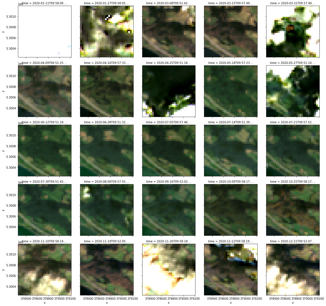
However, we can change the collection if we need to. This is an example using Landsat-8 Collection 2 Level 2 from Planetary Computer:
[3]:
da = cubo.create(
    lat=47.848151988493385,
    lon=13.379491178028564,
    collection="landsat-c2-l2",
    bands=["blue","green","red"],
    start_date="2020-01-01",
    end_date="2021-01-01",
    edge_size=32,
    resolution=30,
    query={
        "eo:cloud_cover": {"lt": 50},
        "platform": {"eq": "landsat-8"}
    }
)
da
[3]:
<xarray.DataArray 'landsat-c2-l2' (time: 25, band: 3, y: 32, x: 32)>
dask.array<fetch_raster_window, shape=(25, 3, 32, 32), dtype=float64, chunksize=(1, 1, 32, 32), chunktype=numpy.ndarray>
Coordinates: (12/30)
  * time                         (time) datetime64[ns] 2020-01-11T09:58:09.42...
    id                           (time) <U31 'LC08_L2SP_192027_20200111_02_T1...
  * band                         (band) <U5 'blue' 'green' 'red'
  * x                            (x) float64 3.783e+05 3.783e+05 ... 3.792e+05
  * y                            (y) float64 5.301e+06 5.301e+06 ... 5.3e+06
    landsat:cloud_cover_land     (time) float64 44.67 18.59 ... 44.81 42.77
    ...                           ...
    raster:bands                 object {'scale': 2.75e-05, 'nodata': 0, 'off...
    title                        (band) <U10 'Blue Band' 'Green Band' 'Red Band'
    common_name                  (band) <U5 'blue' 'green' 'red'
    center_wavelength            (band) float64 0.48 0.56 0.65
    full_width_half_max          (band) float64 0.06 0.06 0.04
    epsg                         <U10 'EPSG:32633'
Attributes:
    collection:           landsat-c2-l2
    stac:                 https://planetarycomputer.microsoft.com/api/stac/v1
    epsg:                 EPSG:32633
    resolution:           30
    edge_size:            32
    central_lat:          47.848151988493385
    central_lon:          13.379491178028564
    central_y:            5300694.38448788
    central_x:            378764.6058600877
    time_coverage_start:  2020-01-01
    time_coverage_end:    2021-01-01
xarray.DataArray
'landsat-c2-l2'
- time: 25
- band: 3
- y: 32
- x: 32
- dask.array<chunksize=(1, 1, 32, 32), meta=np.ndarray>
Array Chunk Bytes 600.00 kiB 8.00 kiB Shape (25, 3, 32, 32) (1, 1, 32, 32) Count 225 Tasks 75 Chunks Type float64 numpy.ndarray - time(time)datetime64[ns]2020-01-11T09:58:09.423694 ... 2...
array(['2020-01-11T09:58:09.423694000', '2020-01-27T09:58:05.073326000', '2020-03-08T09:51:42.064592000', '2020-03-15T09:57:49.583619000', '2020-03-31T09:57:40.292147000', '2020-04-09T09:51:25.637238000', '2020-04-16T09:57:33.592939000', '2020-04-25T09:51:18.431091000', '2020-05-18T09:57:23.802236000', '2020-05-27T09:51:14.586937000', '2020-06-12T09:51:24.372587000', '2020-06-28T09:51:32.821849000', '2020-07-05T09:57:46.722775000', '2020-07-14T09:51:39.267858000', '2020-07-21T09:57:52.312772000', '2020-07-30T09:51:43.743589000', '2020-08-06T09:57:55.907146000', '2020-09-16T09:52:02.334100000', '2020-10-09T09:58:17.908188000', '2020-10-25T09:58:17.979092000', '2020-11-10T09:58:14.921425000', '2020-11-19T09:52:05.749387000', '2020-11-26T09:58:18.320452000', '2020-12-12T09:58:19.124105000', '2020-12-21T09:52:07.042259000'], dtype='datetime64[ns]') - id(time)<U31'LC08_L2SP_192027_20200111_02_T1...
array(['LC08_L2SP_192027_20200111_02_T1', 'LC08_L2SP_192027_20200127_02_T1', 'LC08_L2SP_191027_20200308_02_T1', 'LC08_L2SP_192027_20200315_02_T1', 'LC08_L2SP_192027_20200331_02_T1', 'LC08_L2SP_191027_20200409_02_T1', 'LC08_L2SP_192027_20200416_02_T1', 'LC08_L2SP_191027_20200425_02_T1', 'LC08_L2SP_192027_20200518_02_T1', 'LC08_L2SP_191027_20200527_02_T1', 'LC08_L2SP_191027_20200612_02_T1', 'LC08_L2SP_191027_20200628_02_T1', 'LC08_L2SP_192027_20200705_02_T1', 'LC08_L2SP_191027_20200714_02_T1', 'LC08_L2SP_192027_20200721_02_T1', 'LC08_L2SP_191027_20200730_02_T1', 'LC08_L2SP_192027_20200806_02_T1', 'LC08_L2SP_191027_20200916_02_T1', 'LC08_L2SP_192027_20201009_02_T1', 'LC08_L2SP_192027_20201025_02_T1', 'LC08_L2SP_192027_20201110_02_T1', 'LC08_L2SP_191027_20201119_02_T1', 'LC08_L2SP_192027_20201126_02_T1', 'LC08_L2SP_192027_20201212_02_T1', 'LC08_L2SP_191027_20201221_02_T1'], dtype='<U31') - band(band)<U5'blue' 'green' 'red'
array(['blue', 'green', 'red'], dtype='<U5')
- x(x)float643.783e+05 3.783e+05 ... 3.792e+05
array([378270., 378300., 378330., 378360., 378390., 378420., 378450., 378480., 378510., 378540., 378570., 378600., 378630., 378660., 378690., 378720., 378750., 378780., 378810., 378840., 378870., 378900., 378930., 378960., 378990., 379020., 379050., 379080., 379110., 379140., 379170., 379200.]) - y(y)float645.301e+06 5.301e+06 ... 5.3e+06
array([5301180., 5301150., 5301120., 5301090., 5301060., 5301030., 5301000., 5300970., 5300940., 5300910., 5300880., 5300850., 5300820., 5300790., 5300760., 5300730., 5300700., 5300670., 5300640., 5300610., 5300580., 5300550., 5300520., 5300490., 5300460., 5300430., 5300400., 5300370., 5300340., 5300310., 5300280., 5300250.]) - landsat:cloud_cover_land(time)float6444.67 18.59 26.79 ... 44.81 42.77
array([44.67, 18.59, 26.79, 18.48, 46.18, 10.84, 12.93, 48.89, 18.97, 33.51, 2.81, 15.58, 12.44, 30.91, 40.21, 14.06, 12.55, 12.32, 26.83, 28.07, 38.1 , 23.46, 29.01, 44.81, 42.77]) - landsat:wrs_path(time)<U3'192' '192' '191' ... '192' '191'
array(['192', '192', '191', '192', '192', '191', '192', '191', '192', '191', '191', '191', '192', '191', '192', '191', '192', '191', '192', '192', '192', '191', '192', '192', '191'], dtype='<U3') - instruments()object{'tirs', 'oli'}
array({'tirs', 'oli'}, dtype=object) - landsat:collection_category()<U2'T1'
array('T1', dtype='<U2') - gsd()int6430
array(30)
- created(time)<U27'2022-05-06T18:00:24.616162Z' .....
array(['2022-05-06T18:00:24.616162Z', '2022-05-06T18:00:24.765229Z', '2022-05-06T16:38:14.214165Z', '2022-05-06T18:00:25.364781Z', '2022-05-06T18:00:25.575811Z', '2022-05-06T16:38:14.565762Z', '2022-05-06T18:00:25.743376Z', '2022-05-06T16:38:14.746909Z', '2022-05-06T18:00:26.183086Z', '2022-05-06T16:38:15.155697Z', '2022-05-06T16:38:15.334943Z', '2022-05-06T16:38:15.505274Z', '2022-05-06T18:00:26.656896Z', '2022-05-06T16:38:15.670883Z', '2022-05-06T18:00:26.841124Z', '2022-05-06T16:38:15.835643Z', '2022-05-06T18:00:26.995134Z', '2022-05-06T16:38:16.348486Z', '2022-05-06T18:00:27.714456Z', '2022-05-06T18:00:27.870359Z', '2022-05-06T18:00:28.039599Z', '2022-05-06T16:38:16.865327Z', '2022-05-06T18:00:28.224001Z', '2022-05-06T18:00:28.423217Z', '2022-05-06T16:38:17.216737Z'], dtype='<U27') - proj:epsg()int6432633
array(32633)
- landsat:wrs_row()<U3'027'
array('027', dtype='<U3') - platform()<U9'landsat-8'
array('landsat-8', dtype='<U9') - view:sun_azimuth(time)float64160.7 158.6 154.7 ... 164.3 163.3
array([160.67266272, 158.57564396, 154.68134151, 154.21816033, 153.16963598, 152.49443249, 151.86775535, 150.87415167, 147.43769037, 145.79475029, 143.09988229, 141.61728251, 141.58388461, 142.13385361, 143.00033387, 144.60901888, 146.17591958, 157.25315185, 162.28907488, 164.51916497, 165.55462928, 165.60620025, 165.40754676, 164.26503791, 163.29052159]) - description(band)<U59'Collection 2 Level-2 Blue Band ...
array(['Collection 2 Level-2 Blue Band (SR_B2) Surface Reflectance', 'Collection 2 Level-2 Green Band (SR_B3) Surface Reflectance', 'Collection 2 Level-2 Red Band (SR_B4) Surface Reflectance'], dtype='<U59') - landsat:scene_id(time)<U21'LC81920272020011LGN00' ... 'LC8...
array(['LC81920272020011LGN00', 'LC81920272020027LGN00', 'LC81910272020068LGN00', 'LC81920272020075LGN00', 'LC81920272020091LGN00', 'LC81910272020100LGN00', 'LC81920272020107LGN00', 'LC81910272020116LGN00', 'LC81920272020139LGN00', 'LC81910272020148LGN00', 'LC81910272020164LGN00', 'LC81910272020180LGN00', 'LC81920272020187LGN00', 'LC81910272020196LGN00', 'LC81920272020203LGN00', 'LC81910272020212LGN00', 'LC81920272020219LGN00', 'LC81910272020260LGN00', 'LC81920272020283LGN00', 'LC81920272020299LGN00', 'LC81920272020315LGN00', 'LC81910272020324LGN00', 'LC81920272020331LGN00', 'LC81920272020347LGN00', 'LC81910272020356LGN00'], dtype='<U21') - view:off_nadir()int640
array(0)
- view:sun_elevation(time)float6418.44 21.35 34.85 ... 17.92 17.4
array([18.44477734, 21.35497679, 34.84596743, 37.61178175, 43.95366883, 47.38643777, 49.92260847, 52.93608344, 58.93845601, 60.44266148, 61.80305294, 61.51082918, 60.91183685, 59.76685173, 58.60749656, 56.80958835, 55.19166155, 42.72194858, 34.51211207, 28.9649906 , 24.05267982, 21.73898572, 20.22888734, 17.9173839 , 17.39861873]) - landsat:collection_number()<U2'02'
array('02', dtype='<U2') - eo:cloud_cover(time)float6444.67 18.59 26.79 ... 44.81 42.77
array([44.67, 18.59, 26.79, 18.48, 46.18, 10.84, 12.93, 48.89, 18.97, 33.51, 2.81, 15.58, 12.44, 30.91, 40.21, 14.06, 12.55, 12.32, 26.83, 28.07, 38.1 , 23.46, 29.01, 44.81, 42.77]) - landsat:correction()<U4'L2SP'
array('L2SP', dtype='<U4') - landsat:wrs_type()<U1'2'
array('2', dtype='<U1') - sci:doi()<U16'10.5066/P9OGBGM6'
array('10.5066/P9OGBGM6', dtype='<U16') - raster:bands()object{'scale': 2.75e-05, 'nodata': 0,...
array({'scale': 2.75e-05, 'nodata': 0, 'offset': -0.2, 'data_type': 'uint16', 'spatial_resolution': 30}, dtype=object) - title(band)<U10'Blue Band' 'Green Band' 'Red Band'
array(['Blue Band', 'Green Band', 'Red Band'], dtype='<U10')
- common_name(band)<U5'blue' 'green' 'red'
array(['blue', 'green', 'red'], dtype='<U5')
- center_wavelength(band)float640.48 0.56 0.65
array([0.48, 0.56, 0.65])
- full_width_half_max(band)float640.06 0.06 0.04
array([0.06, 0.06, 0.04])
- epsg()<U10'EPSG:32633'
array('EPSG:32633', dtype='<U10')
- collection :
- landsat-c2-l2
- stac :
- https://planetarycomputer.microsoft.com/api/stac/v1
- epsg :
- EPSG:32633
- resolution :
- 30
- edge_size :
- 32
- central_lat :
- 47.848151988493385
- central_lon :
- 13.379491178028564
- central_y :
- 5300694.38448788
- central_x :
- 378764.6058600877
- time_coverage_start :
- 2020-01-01
- time_coverage_end :
- 2021-01-01
Visualize an RGB image per timestep in the cube:
[4]:
da = (da * 0.0000275) - 0.2
(da.sel(band=["red","green","blue"])/0.2).clip(0,1).plot.imshow(col="time",col_wrap = 5)
[4]:
<xarray.plot.facetgrid.FacetGrid at 0x7f6d62250520>